
1. Decision trees are powerful but rarely used in practice due to their high variance. 2. They are low-bias, high-variance models, and ensemble methods like bagging, boosting, and stacking address these limitations. 3. Ensemble techniques evolve to improve model performance by combining diverse learning strategies.
When studying machine learning, one of the most intuitive yet powerful algorithms you encounter is the Decision Tree. However, in practice—especially in environments like Kaggle competitions—using a single decision tree is rare. Instead, practitioners typically use ensemble models built on top of trees, such as Random Forest or XGBoost.
In this post, we’ll start from the core principles of Decision Trees, explain why they are considered low-bias, high-variance models, and then walk through the evolution of ensemble techniques designed to overcome these limitations: Bagging, Boosting, and Stacking.
1. What is a Decision Tree?
A Decision Tree can be thought of as a game of Twenty Questions.
The model repeatedly asks questions that best separate the data until it arrives at a final prediction.
1.1 Classification vs Regression Trees
Decision Trees are used for two types of tasks depending on the objective.
-
Classification Tree:
-
When the model reaches a leaf node, it predicts the most frequent class (mode) among the training samples in that region.
-
Example: "This region contains 10 tuna and 2 mackerel. A new fish entering this region is most likely tuna." (Majority Voting)
-
-
Regression Tree:
-
In regression tasks, the prediction at a leaf node is the average value (mean) of the target variable among the samples in that region.
-
In other words, the feature space is divided into multiple rectangular regions, and each region is assigned a representative value.
-
1.2 Training Method: Recursive Binary Splitting
The entire training process of a decision tree is called Recursive Binary Splitting.
As the name suggests, the algorithm repeatedly:
-
Splits the data into two parts (binary splitting)
-
Applies the same process recursively (recursive)
At each split, the algorithm uses a greedy strategy, selecting the feature and threshold that most reduces uncertainty (or minimizes loss).
The specific loss function depends on the type of problem.
For every split:
-
A single feature is selected
-
Several candidate thresholds are evaluated
-
The loss is computed for each candidate split
In theory, we could sort all samples and try every possible threshold between values. However, this would dramatically increase computational cost. Modern libraries instead define a fixed number of candidate bins and evaluate splits only at those boundaries.
Another important characteristic:
A decision tree never splits using multiple features simultaneously.
For example, it does not learn rules like: a*x1 + b*x2 > c
Instead, splits always involve a single feature at a time.
If the true decision boundary is diagonal, the tree approximates it using many small step-like splits, creating a staircase-shaped boundary.
Although this seems inefficient, searching for optimal coefficients aaa and bbb would create an almost infinite search space. It is often computationally cheaper to approximate the boundary using multiple splits.
Alternatively, one could use PCA beforehand to combine correlated features.
2. Splitting Criteria
2.1 Classification: Gini Index and Cross-Entropy
In classification problems, trees minimize impurity.
A common measure is the Gini Index:
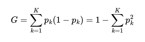
Lower impurity (closer to 0) means the node contains mostly one class.
Another common metric is cross-entropy (log loss).
2.2 Regression: Residual Sum of Squares (RSS)
For regression trees, the objective is to reduce prediction error.
The typical metric is Residual Sum of Squares (RSS):
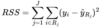
where ![]() is the mean value of the target in region R.
is the mean value of the target in region R.
The algorithm selects the split that produces the largest reduction in RSS.
3. Limitations of Decision Trees
3.1 The Major Problem: Overfitting
If left unconstrained, a decision tree will continue splitting until every leaf contains a single sample.
This leads to two key properties:
-
Low Bias: The model can fit extremely complex patterns.
-
High Variance: Small changes in the training data can produce completely different trees.
In other words, decision trees are very prone to overfitting.
3.2 Solutions: Pruning and Constraints
To prevent overfitting, we apply constraints or pruning techniques.
Pre-Pruning (Early Stopping)
Examples include:
-
max_depth
Limit the maximum depth of the tree (usually tuned via cross-validation). -
min_samples_leaf
Require a minimum number of samples in each leaf node to ensure reliable predictions.
Post-Pruning
Another approach is to grow the tree fully first and then prune unnecessary branches.
One common method is Cost Complexity Pruning:
![]()
where:
-
|T| = number of leaf nodes
-
α = complexity penalty parameter
The algorithm evaluates subtrees and removes branches if the reduction in complexity outweighs the increase in loss.
When α=0, no pruning occurs.
As α increases, the resulting tree becomes simpler.
4. Ensemble Methods: The Power of Collective Intelligence
A single decision tree is unstable due to high variance.
However, combining many trees produces a much stronger model.
This idea leads to Ensemble Learning, which evolved through three major stages:
Bagging → Boosting → Stacking
4.1 Bagging (Bootstrap Aggregation)
The key idea:
Train the same model multiple times on different datasets and average the results.
Step 1: Bootstrap Sampling
Multiple datasets are created by sampling the original dataset with replacement.
Step 2: Aggregation
Each dataset trains an independent tree.
The predictions are then combined.
-
Classification → majority voting
-
Regression → averaging
Effect:
Bagging reduces variance by averaging many unstable models.
4.2 Random Forest
Random Forest is an extension of Bagging.
Even with Bagging, trees may still be similar if a strong feature dominates the splits.
Random Forest introduces feature randomness.
At each split:
-
Instead of considering all features
-
The algorithm randomly selects a subset of features
-
The best split is chosen from that subset
This reduces correlation between trees, increasing diversity and improving performance.
4.3 Boosting (AdaBoost, GBM, XGBoost)
Boosting differs from Bagging because models are trained sequentially rather than independently.
The core idea:
Each model focuses on correcting the mistakes of the previous model.
AdaBoost
-
Samples that were misclassified receive higher weights.
-
The next model focuses more on those difficult samples.
Final predictions are a weighted sum of all models, where each model’s weight reflects its reliability.
Gradient Boosting and XGBoost
The key concept is Residual Learning.
Training proceeds as follows:
-
Model 1 predicts y
-
Compute residuals r1
-
Model 2 learns to predict r1
-
Compute new residuals r2
-
Model 3 predicts r2
The final prediction is the sum of all model outputs.
![]()
In practice:
-
The base score is the mean of the training labels.
-
The first model effectively learns y_true - average.
The residual corresponds to the gradient of the loss function, which is why this method is called Gradient Boosting.
XGBoost Hyperparameter Tips
Common settings include:
-
n_estimators
Number of trees. -
learning_rate
Controls how much each new tree contributes (smaller values help prevent overfitting). -
max_depth
Boosting trees are usually shallow weak learners (typically depth 3–6).
This contrasts with Random Forest, where trees are often grown deeper.
5. Stacking
Stacking combines different types of models.
For example:
-
SVM
-
Decision Trees
-
KNN
Each model produces predictions, and those predictions become features for a meta learner.
The meta learner (often a simple linear regression) learns how to best combine them.
Stacking is frequently used in top Kaggle solutions to squeeze out the final fraction of performance.
Summary Cheat Sheet
| Model | Core Idea | Training Style | Bias / Variance | Tree Depth |
|---|---|---|---|---|
| Decision Tree | Greedy splitting | Single model | Low Bias / High Variance | Can grow very deep |
| Random Forest | Bagging + feature randomness | Parallel independent trees | Strong variance reduction | Usually deep |
| Gradient Boosting (XGB) | Residual learning | Sequential | Strong bias reduction | Usually shallow |
Final Thoughts
Machine learning modeling is fundamentally a trade-off between:
-
Bias: how well a model captures patterns in the data
-
Variance: how sensitive the model is to changes in the training data
Decision Trees are the starting point.
Understanding how ensemble methods evolved to address their weaknesses provides valuable insight into designing more powerful models.
Python Example
from sklearn.tree import DecisionTreeClassifier
from sklearn.ensemble import RandomForestClassifier, GradientBoostingClassifier
import xgboost as xgb

# 1. Decision Tree
dt = DecisionTreeClassifier(max_depth=5, random_state=42)
dt.fit(X_train, y_train)

# 2. Random Forest (Bagging)
rf = RandomForestClassifier(n_estimators=100, max_depth=None, random_state=42)
rf.fit(X_train, y_train)

# 3. XGBoost (Boosting)
xgb_model = xgb.XGBClassifier(
    n_estimators=1000,
    learning_rate=0.1,
    max_depth=3,
    random_state=42
)
xgb_model.fit(X_train, y_train)